{
 "cells": [
  {
   "cell_type": "markdown",
   "id": "1e25f29b",
   "metadata": {},
   "source": [
    "#  Lecture 04. Data Aggregation and Group Operations\n",
    "\n",
    "### Instructor: Luping Yu\n",
    "\n",
    "### Mar 19, 2024\n",
    "\n",
    "***\n",
    "\n",
    "Categorizing a dataset and applying a function to each group, whether an **aggregation** or **transformation**, is often a critical component of a data analysis workflow. After loading and preparing a dataset, you may need to compute group statistics for reporting or visualization purposes.\n",
    "\n",
    "<code>pandas</code> provides a flexible <code>groupby()</code> interface, enabling you to slice, dice, and summarize datasets in a natural way.\n",
    "\n",
    "***\n",
    "### GroupBy Mechanics\n",
    "\n",
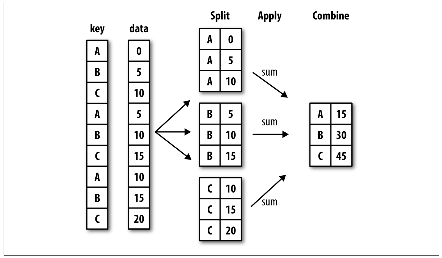
    "Punchline: **split-apply-combine （拆分-应用-合并）** \n",
    "* In the first stage of the process, data is **split** into groups based on one or more keys that you provide.\n",
    "* Once this is done, a function is **applied** to each group, producing a new value.\n",
    "* Finally, the results of all those function applications are **combined** into a result object.\n",
    "\n",
    "See the following figure for a mockup of a simple group aggregation:\n",
    "\n",
    "![avatar](https://raw.githubusercontent.com/lazydingding/gallery/main/Screen%20Shot%202022-03-14%20at%2022.58.22.png)\n",
    "***\n",
    "\n",
    "To get started, here is a small tabular dataset as a <code>DataFrame</code>:"
   ]
  },
  {
   "cell_type": "code",
   "execution_count": 1,
   "id": "7e30f646",
   "metadata": {},
   "outputs": [
    {
     "data": {
      "text/html": [
       "<div>\n",
       "<style scoped>\n",
       "    .dataframe tbody tr th:only-of-type {\n",
       "        vertical-align: middle;\n",
       "    }\n",
       "\n",
       "    .dataframe tbody tr th {\n",
       "        vertical-align: top;\n",
       "    }\n",
       "\n",
       "    .dataframe thead th {\n",
       "        text-align: right;\n",
       "    }\n",
       "</style>\n",
       "<table border=\"1\" class=\"dataframe\">\n",
       "  <thead>\n",
       "    <tr style=\"text-align: right;\">\n",
       "      <th></th>\n",
       "      <th>key1</th>\n",
       "      <th>key2</th>\n",
       "      <th>data1</th>\n",
       "      <th>data2</th>\n",
       "    </tr>\n",
       "  </thead>\n",
       "  <tbody>\n",
       "    <tr>\n",
       "      <th>0</th>\n",
       "      <td>a</td>\n",
       "      <td>one</td>\n",
       "      <td>-1.137953</td>\n",
       "      <td>-1.741685</td>\n",
       "    </tr>\n",
       "    <tr>\n",
       "      <th>1</th>\n",
       "      <td>a</td>\n",
       "      <td>two</td>\n",
       "      <td>0.014705</td>\n",
       "      <td>-0.937821</td>\n",
       "    </tr>\n",
       "    <tr>\n",
       "      <th>2</th>\n",
       "      <td>b</td>\n",
       "      <td>one</td>\n",
       "      <td>0.140717</td>\n",
       "      <td>-0.420972</td>\n",
       "    </tr>\n",
       "    <tr>\n",
       "      <th>3</th>\n",
       "      <td>b</td>\n",
       "      <td>two</td>\n",
       "      <td>-0.098441</td>\n",
       "      <td>0.548059</td>\n",
       "    </tr>\n",
       "    <tr>\n",
       "      <th>4</th>\n",
       "      <td>a</td>\n",
       "      <td>one</td>\n",
       "      <td>-1.203151</td>\n",
       "      <td>-0.664293</td>\n",
       "    </tr>\n",
       "  </tbody>\n",
       "</table>\n",
       "</div>"
      ],
      "text/plain": [
       "  key1 key2     data1     data2\n",
       "0    a  one -1.137953 -1.741685\n",
       "1    a  two  0.014705 -0.937821\n",
       "2    b  one  0.140717 -0.420972\n",
       "3    b  two -0.098441  0.548059\n",
       "4    a  one -1.203151 -0.664293"
      ]
     },
     "execution_count": 1,
     "metadata": {},
     "output_type": "execute_result"
    }
   ],
   "source": [
    "import pandas as pd\n",
    "import numpy as np\n",
    "#np.random.randn: generate random numbers\n",
    "\n",
    "df = pd.DataFrame({'key1' : ['a', 'a', 'b', 'b', 'a'],\n",
    "                   'key2' : ['one', 'two', 'one', 'two', 'one'],\n",
    "                   'data1' : np.random.randn(5),\n",
    "                   'data2' : np.random.randn(5)})\n",
    "\n",
    "df"
   ]
  },
  {
   "cell_type": "markdown",
   "id": "1c82534a",
   "metadata": {},
   "source": [
    "Suppose you wanted to compute the **mean** of the <code>data1</code> column using the labels from <code>key1</code>.\n",
    "\n",
    "There are a number of ways to do this. One is to access <code>data1</code> and call <code>groupby()</code> with the column at <code>key1</code>:"
   ]
  },
  {
   "cell_type": "code",
   "execution_count": 2,
   "id": "4235891d",
   "metadata": {},
   "outputs": [
    {
     "data": {
      "text/plain": [
       "<pandas.core.groupby.generic.SeriesGroupBy object at 0x111d9dad0>"
      ]
     },
     "execution_count": 2,
     "metadata": {},
     "output_type": "execute_result"
    }
   ],
   "source": [
    "grouped = df['data1'].groupby(df['key1'])\n",
    "\n",
    "grouped"
   ]
  },
  {
   "cell_type": "markdown",
   "id": "42d2a5c6",
   "metadata": {},
   "source": [
    "This grouped variable is now a <code>GroupBy object</code>.\n",
    "\n",
    "It has not actually computed anything yet except for some intermediate data about the group key <code>df['key1']</code>. The idea is that this object has all of the information needed to then apply some operation to each of the groups.\n",
    "\n",
    "For example, to compute group means we can call the GroupBy's <code>mean()</code> method:"
   ]
  },
  {
   "cell_type": "code",
   "execution_count": 3,
   "id": "2225746f",
   "metadata": {
    "scrolled": true
   },
   "outputs": [
    {
     "data": {
      "text/plain": [
       "key1\n",
       "a   -0.775467\n",
       "b    0.021138\n",
       "Name: data1, dtype: float64"
      ]
     },
     "execution_count": 3,
     "metadata": {},
     "output_type": "execute_result"
    }
   ],
   "source": [
    "grouped.mean()"
   ]
  },
  {
   "cell_type": "markdown",
   "id": "f00cb2a9",
   "metadata": {},
   "source": [
    "The important thing here is that the data has been **aggregated** according to the group key, producing a new Series that is now indexed by the **unique values** in the <code>key1</code> column.\n",
    "\n",
    "If instead we had passed multiple arrays as a list, we'd get something different:"
   ]
  },
  {
   "cell_type": "code",
   "execution_count": 4,
   "id": "ef277cb1",
   "metadata": {
    "scrolled": true
   },
   "outputs": [
    {
     "data": {
      "text/plain": [
       "key1  key2\n",
       "a     one    -1.170552\n",
       "      two     0.014705\n",
       "b     one     0.140717\n",
       "      two    -0.098441\n",
       "Name: data1, dtype: float64"
      ]
     },
     "execution_count": 4,
     "metadata": {},
     "output_type": "execute_result"
    }
   ],
   "source": [
    "df['data1'].groupby([df['key1'], df['key2']]).mean()"
   ]
  },
  {
   "cell_type": "markdown",
   "id": "dac70643",
   "metadata": {},
   "source": [
    "Here we grouped the data using **two keys**, and the resulting Series now has a **hierarchical index** consisting of the **unique pairs** of keys observed.\n",
    "\n",
    "A generally useful GroupBy method is <code>size()</code>, which returns a Series containing group sizes:"
   ]
  },
  {
   "cell_type": "code",
   "execution_count": 5,
   "id": "3fecc78e",
   "metadata": {
    "scrolled": true
   },
   "outputs": [
    {
     "data": {
      "text/plain": [
       "key1  key2\n",
       "a     one     2\n",
       "      two     1\n",
       "b     one     1\n",
       "      two     1\n",
       "dtype: int64"
      ]
     },
     "execution_count": 5,
     "metadata": {},
     "output_type": "execute_result"
    }
   ],
   "source": [
    "df.groupby(['key1', 'key2']).size()"
   ]
  },
  {
   "cell_type": "markdown",
   "id": "71211471",
   "metadata": {},
   "source": [
    "For large datasets, it may be desirable to aggregate only a few columns. For example, in the preceding dataset, to compute means for just the <code>data2</code> column, we could write:"
   ]
  },
  {
   "cell_type": "code",
   "execution_count": 6,
   "id": "cffb413c",
   "metadata": {
    "scrolled": true
   },
   "outputs": [
    {
     "data": {
      "text/plain": [
       "key1  key2\n",
       "a     one    -1.202989\n",
       "      two    -0.937821\n",
       "b     one    -0.420972\n",
       "      two     0.548059\n",
       "Name: data2, dtype: float64"
      ]
     },
     "execution_count": 6,
     "metadata": {},
     "output_type": "execute_result"
    }
   ],
   "source": [
    "df.groupby(['key1', 'key2'])['data2'].mean()"
   ]
  },
  {
   "cell_type": "markdown",
   "id": "c2c45ba4",
   "metadata": {},
   "source": [
    "***\n",
    "\n",
    "### Data Aggregation\n",
    "\n",
    "**Aggregations** refer to any data transformation that produces scalar values from arrays. The preceding examples have used several of them, including <code>mean</code> and <code>size</code>. Built-in functions can be invoked using <code>agg()</code>.\n",
    "\n",
    "|Function | Description |\n",
    "|:- | :- | \n",
    "|count | Number of non-NA values in the group\n",
    "|sum | Sum of non-NA values\n",
    "|mean | Mean of non-NA values\n",
    "|median | Arithmetic median of non-NA values\n",
    "|std, var | Unbiased (n – 1 denominator) standard deviation and variance\n",
    "|min, max | Minimum and maximum of non-NA values\n",
    "|first, last | First and last non-NA values\n"
   ]
  },
  {
   "cell_type": "code",
   "execution_count": 7,
   "id": "64083577",
   "metadata": {
    "scrolled": true
   },
   "outputs": [
    {
     "data": {
      "text/html": [
       "<div>\n",
       "<style scoped>\n",
       "    .dataframe tbody tr th:only-of-type {\n",
       "        vertical-align: middle;\n",
       "    }\n",
       "\n",
       "    .dataframe tbody tr th {\n",
       "        vertical-align: top;\n",
       "    }\n",
       "\n",
       "    .dataframe thead th {\n",
       "        text-align: right;\n",
       "    }\n",
       "</style>\n",
       "<table border=\"1\" class=\"dataframe\">\n",
       "  <thead>\n",
       "    <tr style=\"text-align: right;\">\n",
       "      <th></th>\n",
       "      <th>key1</th>\n",
       "      <th>data1</th>\n",
       "      <th>data2</th>\n",
       "    </tr>\n",
       "  </thead>\n",
       "  <tbody>\n",
       "    <tr>\n",
       "      <th>0</th>\n",
       "      <td>a</td>\n",
       "      <td>-1.137953</td>\n",
       "      <td>-1.741685</td>\n",
       "    </tr>\n",
       "    <tr>\n",
       "      <th>1</th>\n",
       "      <td>a</td>\n",
       "      <td>0.014705</td>\n",
       "      <td>-0.937821</td>\n",
       "    </tr>\n",
       "    <tr>\n",
       "      <th>2</th>\n",
       "      <td>b</td>\n",
       "      <td>0.140717</td>\n",
       "      <td>-0.420972</td>\n",
       "    </tr>\n",
       "    <tr>\n",
       "      <th>3</th>\n",
       "      <td>b</td>\n",
       "      <td>-0.098441</td>\n",
       "      <td>0.548059</td>\n",
       "    </tr>\n",
       "    <tr>\n",
       "      <th>4</th>\n",
       "      <td>a</td>\n",
       "      <td>-1.203151</td>\n",
       "      <td>-0.664293</td>\n",
       "    </tr>\n",
       "  </tbody>\n",
       "</table>\n",
       "</div>"
      ],
      "text/plain": [
       "  key1     data1     data2\n",
       "0    a -1.137953 -1.741685\n",
       "1    a  0.014705 -0.937821\n",
       "2    b  0.140717 -0.420972\n",
       "3    b -0.098441  0.548059\n",
       "4    a -1.203151 -0.664293"
      ]
     },
     "execution_count": 7,
     "metadata": {},
     "output_type": "execute_result"
    }
   ],
   "source": [
    "df = df[['key1','data1','data2']]\n",
    "\n",
    "df"
   ]
  },
  {
   "cell_type": "code",
   "execution_count": 8,
   "id": "2ea90a13",
   "metadata": {},
   "outputs": [
    {
     "data": {
      "text/html": [
       "<div>\n",
       "<style scoped>\n",
       "    .dataframe tbody tr th:only-of-type {\n",
       "        vertical-align: middle;\n",
       "    }\n",
       "\n",
       "    .dataframe tbody tr th {\n",
       "        vertical-align: top;\n",
       "    }\n",
       "\n",
       "    .dataframe thead th {\n",
       "        text-align: right;\n",
       "    }\n",
       "</style>\n",
       "<table border=\"1\" class=\"dataframe\">\n",
       "  <thead>\n",
       "    <tr style=\"text-align: right;\">\n",
       "      <th></th>\n",
       "      <th>data1</th>\n",
       "      <th>data2</th>\n",
       "    </tr>\n",
       "    <tr>\n",
       "      <th>key1</th>\n",
       "      <th></th>\n",
       "      <th></th>\n",
       "    </tr>\n",
       "  </thead>\n",
       "  <tbody>\n",
       "    <tr>\n",
       "      <th>a</th>\n",
       "      <td>0.014705</td>\n",
       "      <td>-0.664293</td>\n",
       "    </tr>\n",
       "    <tr>\n",
       "      <th>b</th>\n",
       "      <td>0.140717</td>\n",
       "      <td>0.548059</td>\n",
       "    </tr>\n",
       "  </tbody>\n",
       "</table>\n",
       "</div>"
      ],
      "text/plain": [
       "         data1     data2\n",
       "key1                    \n",
       "a     0.014705 -0.664293\n",
       "b     0.140717  0.548059"
      ]
     },
     "execution_count": 8,
     "metadata": {},
     "output_type": "execute_result"
    }
   ],
   "source": [
    "df.groupby('key1').max()"
   ]
  },
  {
   "cell_type": "code",
   "execution_count": 9,
   "id": "a183aa7d",
   "metadata": {},
   "outputs": [
    {
     "data": {
      "text/html": [
       "<div>\n",
       "<style scoped>\n",
       "    .dataframe tbody tr th:only-of-type {\n",
       "        vertical-align: middle;\n",
       "    }\n",
       "\n",
       "    .dataframe tbody tr th {\n",
       "        vertical-align: top;\n",
       "    }\n",
       "\n",
       "    .dataframe thead th {\n",
       "        text-align: right;\n",
       "    }\n",
       "</style>\n",
       "<table border=\"1\" class=\"dataframe\">\n",
       "  <thead>\n",
       "    <tr style=\"text-align: right;\">\n",
       "      <th></th>\n",
       "      <th>data1</th>\n",
       "      <th>data2</th>\n",
       "    </tr>\n",
       "    <tr>\n",
       "      <th>key1</th>\n",
       "      <th></th>\n",
       "      <th></th>\n",
       "    </tr>\n",
       "  </thead>\n",
       "  <tbody>\n",
       "    <tr>\n",
       "      <th>a</th>\n",
       "      <td>-1.203151</td>\n",
       "      <td>-1.741685</td>\n",
       "    </tr>\n",
       "    <tr>\n",
       "      <th>b</th>\n",
       "      <td>-0.098441</td>\n",
       "      <td>-0.420972</td>\n",
       "    </tr>\n",
       "  </tbody>\n",
       "</table>\n",
       "</div>"
      ],
      "text/plain": [
       "         data1     data2\n",
       "key1                    \n",
       "a    -1.203151 -1.741685\n",
       "b    -0.098441 -0.420972"
      ]
     },
     "execution_count": 9,
     "metadata": {},
     "output_type": "execute_result"
    }
   ],
   "source": [
    "df.groupby('key1').agg('min')"
   ]
  },
  {
   "cell_type": "markdown",
   "id": "81db68a7",
   "metadata": {},
   "source": [
    "To use your own aggregation functions, pass any function that aggregates an array to the <code>apply</code> method:"
   ]
  },
  {
   "cell_type": "code",
   "execution_count": 10,
   "id": "778c3d27",
   "metadata": {},
   "outputs": [],
   "source": [
    "def peak_to_peak(arr):\n",
    "    return arr.max() - arr.min()"
   ]
  },
  {
   "cell_type": "code",
   "execution_count": 11,
   "id": "3dde8c29",
   "metadata": {},
   "outputs": [
    {
     "data": {
      "text/html": [
       "<div>\n",
       "<style scoped>\n",
       "    .dataframe tbody tr th:only-of-type {\n",
       "        vertical-align: middle;\n",
       "    }\n",
       "\n",
       "    .dataframe tbody tr th {\n",
       "        vertical-align: top;\n",
       "    }\n",
       "\n",
       "    .dataframe thead th {\n",
       "        text-align: right;\n",
       "    }\n",
       "</style>\n",
       "<table border=\"1\" class=\"dataframe\">\n",
       "  <thead>\n",
       "    <tr style=\"text-align: right;\">\n",
       "      <th></th>\n",
       "      <th>data1</th>\n",
       "      <th>data2</th>\n",
       "    </tr>\n",
       "    <tr>\n",
       "      <th>key1</th>\n",
       "      <th></th>\n",
       "      <th></th>\n",
       "    </tr>\n",
       "  </thead>\n",
       "  <tbody>\n",
       "    <tr>\n",
       "      <th>a</th>\n",
       "      <td>1.217856</td>\n",
       "      <td>1.077392</td>\n",
       "    </tr>\n",
       "    <tr>\n",
       "      <th>b</th>\n",
       "      <td>0.239158</td>\n",
       "      <td>0.969030</td>\n",
       "    </tr>\n",
       "  </tbody>\n",
       "</table>\n",
       "</div>"
      ],
      "text/plain": [
       "         data1     data2\n",
       "key1                    \n",
       "a     1.217856  1.077392\n",
       "b     0.239158  0.969030"
      ]
     },
     "execution_count": 11,
     "metadata": {},
     "output_type": "execute_result"
    }
   ],
   "source": [
    "df.groupby(df['key1']).apply(peak_to_peak)"
   ]
  },
  {
   "cell_type": "markdown",
   "id": "c5e10b9b",
   "metadata": {},
   "source": [
    "***\n",
    "\n",
    "### General split-apply-combine\n",
    "\n",
    "* Create analysis with <code>.groupby()</code> and **built-in** functions (<code>mean</code>, <code>sum</code>, <code>count</code>, etc.)\n",
    "* Create analysis with <code>.groupby()</code> and user defined functions\n",
    "* Use <code>.transform()</code> to join group stats to the original dataframe\n",
    "\n",
    "Let's get started with the tipping dataset:"
   ]
  },
  {
   "cell_type": "code",
   "execution_count": 12,
   "id": "3cdb9e0b",
   "metadata": {
    "scrolled": true
   },
   "outputs": [
    {
     "data": {
      "text/html": [
       "<div>\n",
       "<style scoped>\n",
       "    .dataframe tbody tr th:only-of-type {\n",
       "        vertical-align: middle;\n",
       "    }\n",
       "\n",
       "    .dataframe tbody tr th {\n",
       "        vertical-align: top;\n",
       "    }\n",
       "\n",
       "    .dataframe thead th {\n",
       "        text-align: right;\n",
       "    }\n",
       "</style>\n",
       "<table border=\"1\" class=\"dataframe\">\n",
       "  <thead>\n",
       "    <tr style=\"text-align: right;\">\n",
       "      <th></th>\n",
       "      <th>day</th>\n",
       "      <th>size</th>\n",
       "      <th>total_bill</th>\n",
       "      <th>tip</th>\n",
       "    </tr>\n",
       "  </thead>\n",
       "  <tbody>\n",
       "    <tr>\n",
       "      <th>0</th>\n",
       "      <td>Sun</td>\n",
       "      <td>2</td>\n",
       "      <td>16.99</td>\n",
       "      <td>1.01</td>\n",
       "    </tr>\n",
       "    <tr>\n",
       "      <th>1</th>\n",
       "      <td>Sun</td>\n",
       "      <td>3</td>\n",
       "      <td>10.34</td>\n",
       "      <td>1.66</td>\n",
       "    </tr>\n",
       "    <tr>\n",
       "      <th>2</th>\n",
       "      <td>Sun</td>\n",
       "      <td>3</td>\n",
       "      <td>21.01</td>\n",
       "      <td>3.50</td>\n",
       "    </tr>\n",
       "    <tr>\n",
       "      <th>3</th>\n",
       "      <td>Sun</td>\n",
       "      <td>2</td>\n",
       "      <td>23.68</td>\n",
       "      <td>3.31</td>\n",
       "    </tr>\n",
       "    <tr>\n",
       "      <th>4</th>\n",
       "      <td>Sun</td>\n",
       "      <td>4</td>\n",
       "      <td>24.59</td>\n",
       "      <td>3.61</td>\n",
       "    </tr>\n",
       "    <tr>\n",
       "      <th>...</th>\n",
       "      <td>...</td>\n",
       "      <td>...</td>\n",
       "      <td>...</td>\n",
       "      <td>...</td>\n",
       "    </tr>\n",
       "    <tr>\n",
       "      <th>239</th>\n",
       "      <td>Sat</td>\n",
       "      <td>3</td>\n",
       "      <td>29.03</td>\n",
       "      <td>5.92</td>\n",
       "    </tr>\n",
       "    <tr>\n",
       "      <th>240</th>\n",
       "      <td>Sat</td>\n",
       "      <td>2</td>\n",
       "      <td>27.18</td>\n",
       "      <td>2.00</td>\n",
       "    </tr>\n",
       "    <tr>\n",
       "      <th>241</th>\n",
       "      <td>Sat</td>\n",
       "      <td>2</td>\n",
       "      <td>22.67</td>\n",
       "      <td>2.00</td>\n",
       "    </tr>\n",
       "    <tr>\n",
       "      <th>242</th>\n",
       "      <td>Sat</td>\n",
       "      <td>2</td>\n",
       "      <td>17.82</td>\n",
       "      <td>1.75</td>\n",
       "    </tr>\n",
       "    <tr>\n",
       "      <th>243</th>\n",
       "      <td>Thur</td>\n",
       "      <td>2</td>\n",
       "      <td>18.78</td>\n",
       "      <td>3.00</td>\n",
       "    </tr>\n",
       "  </tbody>\n",
       "</table>\n",
       "<p>244 rows × 4 columns</p>\n",
       "</div>"
      ],
      "text/plain": [
       "      day  size  total_bill   tip\n",
       "0     Sun     2       16.99  1.01\n",
       "1     Sun     3       10.34  1.66\n",
       "2     Sun     3       21.01  3.50\n",
       "3     Sun     2       23.68  3.31\n",
       "4     Sun     4       24.59  3.61\n",
       "..    ...   ...         ...   ...\n",
       "239   Sat     3       29.03  5.92\n",
       "240   Sat     2       27.18  2.00\n",
       "241   Sat     2       22.67  2.00\n",
       "242   Sat     2       17.82  1.75\n",
       "243  Thur     2       18.78  3.00\n",
       "\n",
       "[244 rows x 4 columns]"
      ]
     },
     "execution_count": 12,
     "metadata": {},
     "output_type": "execute_result"
    }
   ],
   "source": [
    "df = pd.read_csv('examples/tips.csv')\n",
    "\n",
    "df = df[['day','size','total_bill','tip']]\n",
    "\n",
    "df"
   ]
  },
  {
   "cell_type": "code",
   "execution_count": 13,
   "id": "38f4e5da",
   "metadata": {
    "scrolled": true
   },
   "outputs": [
    {
     "data": {
      "text/html": [
       "<div>\n",
       "<style scoped>\n",
       "    .dataframe tbody tr th:only-of-type {\n",
       "        vertical-align: middle;\n",
       "    }\n",
       "\n",
       "    .dataframe tbody tr th {\n",
       "        vertical-align: top;\n",
       "    }\n",
       "\n",
       "    .dataframe thead th {\n",
       "        text-align: right;\n",
       "    }\n",
       "</style>\n",
       "<table border=\"1\" class=\"dataframe\">\n",
       "  <thead>\n",
       "    <tr style=\"text-align: right;\">\n",
       "      <th></th>\n",
       "      <th>size</th>\n",
       "      <th>total_bill</th>\n",
       "      <th>tip</th>\n",
       "    </tr>\n",
       "    <tr>\n",
       "      <th>day</th>\n",
       "      <th></th>\n",
       "      <th></th>\n",
       "      <th></th>\n",
       "    </tr>\n",
       "  </thead>\n",
       "  <tbody>\n",
       "    <tr>\n",
       "      <th>Fri</th>\n",
       "      <td>2.105263</td>\n",
       "      <td>17.151579</td>\n",
       "      <td>2.734737</td>\n",
       "    </tr>\n",
       "    <tr>\n",
       "      <th>Sat</th>\n",
       "      <td>2.517241</td>\n",
       "      <td>20.441379</td>\n",
       "      <td>2.993103</td>\n",
       "    </tr>\n",
       "    <tr>\n",
       "      <th>Sun</th>\n",
       "      <td>2.842105</td>\n",
       "      <td>21.410000</td>\n",
       "      <td>3.255132</td>\n",
       "    </tr>\n",
       "    <tr>\n",
       "      <th>Thur</th>\n",
       "      <td>2.451613</td>\n",
       "      <td>17.682742</td>\n",
       "      <td>2.771452</td>\n",
       "    </tr>\n",
       "  </tbody>\n",
       "</table>\n",
       "</div>"
      ],
      "text/plain": [
       "          size  total_bill       tip\n",
       "day                                 \n",
       "Fri   2.105263   17.151579  2.734737\n",
       "Sat   2.517241   20.441379  2.993103\n",
       "Sun   2.842105   21.410000  3.255132\n",
       "Thur  2.451613   17.682742  2.771452"
      ]
     },
     "execution_count": 13,
     "metadata": {},
     "output_type": "execute_result"
    }
   ],
   "source": [
    "df.groupby('day').mean()"
   ]
  },
  {
   "cell_type": "code",
   "execution_count": 14,
   "id": "44b758df",
   "metadata": {},
   "outputs": [
    {
     "data": {
      "text/html": [
       "<div>\n",
       "<style scoped>\n",
       "    .dataframe tbody tr th:only-of-type {\n",
       "        vertical-align: middle;\n",
       "    }\n",
       "\n",
       "    .dataframe tbody tr th {\n",
       "        vertical-align: top;\n",
       "    }\n",
       "\n",
       "    .dataframe thead th {\n",
       "        text-align: right;\n",
       "    }\n",
       "</style>\n",
       "<table border=\"1\" class=\"dataframe\">\n",
       "  <thead>\n",
       "    <tr style=\"text-align: right;\">\n",
       "      <th></th>\n",
       "      <th>size</th>\n",
       "      <th>total_bill</th>\n",
       "      <th>tip</th>\n",
       "    </tr>\n",
       "  </thead>\n",
       "  <tbody>\n",
       "    <tr>\n",
       "      <th>0</th>\n",
       "      <td>2.842105</td>\n",
       "      <td>21.410000</td>\n",
       "      <td>3.255132</td>\n",
       "    </tr>\n",
       "    <tr>\n",
       "      <th>1</th>\n",
       "      <td>2.842105</td>\n",
       "      <td>21.410000</td>\n",
       "      <td>3.255132</td>\n",
       "    </tr>\n",
       "    <tr>\n",
       "      <th>2</th>\n",
       "      <td>2.842105</td>\n",
       "      <td>21.410000</td>\n",
       "      <td>3.255132</td>\n",
       "    </tr>\n",
       "    <tr>\n",
       "      <th>3</th>\n",
       "      <td>2.842105</td>\n",
       "      <td>21.410000</td>\n",
       "      <td>3.255132</td>\n",
       "    </tr>\n",
       "    <tr>\n",
       "      <th>4</th>\n",
       "      <td>2.842105</td>\n",
       "      <td>21.410000</td>\n",
       "      <td>3.255132</td>\n",
       "    </tr>\n",
       "    <tr>\n",
       "      <th>...</th>\n",
       "      <td>...</td>\n",
       "      <td>...</td>\n",
       "      <td>...</td>\n",
       "    </tr>\n",
       "    <tr>\n",
       "      <th>239</th>\n",
       "      <td>2.517241</td>\n",
       "      <td>20.441379</td>\n",
       "      <td>2.993103</td>\n",
       "    </tr>\n",
       "    <tr>\n",
       "      <th>240</th>\n",
       "      <td>2.517241</td>\n",
       "      <td>20.441379</td>\n",
       "      <td>2.993103</td>\n",
       "    </tr>\n",
       "    <tr>\n",
       "      <th>241</th>\n",
       "      <td>2.517241</td>\n",
       "      <td>20.441379</td>\n",
       "      <td>2.993103</td>\n",
       "    </tr>\n",
       "    <tr>\n",
       "      <th>242</th>\n",
       "      <td>2.517241</td>\n",
       "      <td>20.441379</td>\n",
       "      <td>2.993103</td>\n",
       "    </tr>\n",
       "    <tr>\n",
       "      <th>243</th>\n",
       "      <td>2.451613</td>\n",
       "      <td>17.682742</td>\n",
       "      <td>2.771452</td>\n",
       "    </tr>\n",
       "  </tbody>\n",
       "</table>\n",
       "<p>244 rows × 3 columns</p>\n",
       "</div>"
      ],
      "text/plain": [
       "         size  total_bill       tip\n",
       "0    2.842105   21.410000  3.255132\n",
       "1    2.842105   21.410000  3.255132\n",
       "2    2.842105   21.410000  3.255132\n",
       "3    2.842105   21.410000  3.255132\n",
       "4    2.842105   21.410000  3.255132\n",
       "..        ...         ...       ...\n",
       "239  2.517241   20.441379  2.993103\n",
       "240  2.517241   20.441379  2.993103\n",
       "241  2.517241   20.441379  2.993103\n",
       "242  2.517241   20.441379  2.993103\n",
       "243  2.451613   17.682742  2.771452\n",
       "\n",
       "[244 rows x 3 columns]"
      ]
     },
     "execution_count": 14,
     "metadata": {},
     "output_type": "execute_result"
    }
   ],
   "source": [
    "df.groupby('day').transform('mean')"
   ]
  },
  {
   "cell_type": "code",
   "execution_count": 15,
   "id": "2dec97b7",
   "metadata": {
    "scrolled": true
   },
   "outputs": [
    {
     "data": {
      "text/html": [
       "<div>\n",
       "<style scoped>\n",
       "    .dataframe tbody tr th:only-of-type {\n",
       "        vertical-align: middle;\n",
       "    }\n",
       "\n",
       "    .dataframe tbody tr th {\n",
       "        vertical-align: top;\n",
       "    }\n",
       "\n",
       "    .dataframe thead th {\n",
       "        text-align: right;\n",
       "    }\n",
       "</style>\n",
       "<table border=\"1\" class=\"dataframe\">\n",
       "  <thead>\n",
       "    <tr style=\"text-align: right;\">\n",
       "      <th></th>\n",
       "      <th>day</th>\n",
       "      <th>size</th>\n",
       "      <th>total_bill</th>\n",
       "      <th>tip</th>\n",
       "      <th>day_avg_tip</th>\n",
       "    </tr>\n",
       "  </thead>\n",
       "  <tbody>\n",
       "    <tr>\n",
       "      <th>0</th>\n",
       "      <td>Sun</td>\n",
       "      <td>2</td>\n",
       "      <td>16.99</td>\n",
       "      <td>1.01</td>\n",
       "      <td>3.255132</td>\n",
       "    </tr>\n",
       "    <tr>\n",
       "      <th>1</th>\n",
       "      <td>Sun</td>\n",
       "      <td>3</td>\n",
       "      <td>10.34</td>\n",
       "      <td>1.66</td>\n",
       "      <td>3.255132</td>\n",
       "    </tr>\n",
       "    <tr>\n",
       "      <th>2</th>\n",
       "      <td>Sun</td>\n",
       "      <td>3</td>\n",
       "      <td>21.01</td>\n",
       "      <td>3.50</td>\n",
       "      <td>3.255132</td>\n",
       "    </tr>\n",
       "    <tr>\n",
       "      <th>3</th>\n",
       "      <td>Sun</td>\n",
       "      <td>2</td>\n",
       "      <td>23.68</td>\n",
       "      <td>3.31</td>\n",
       "      <td>3.255132</td>\n",
       "    </tr>\n",
       "    <tr>\n",
       "      <th>4</th>\n",
       "      <td>Sun</td>\n",
       "      <td>4</td>\n",
       "      <td>24.59</td>\n",
       "      <td>3.61</td>\n",
       "      <td>3.255132</td>\n",
       "    </tr>\n",
       "    <tr>\n",
       "      <th>...</th>\n",
       "      <td>...</td>\n",
       "      <td>...</td>\n",
       "      <td>...</td>\n",
       "      <td>...</td>\n",
       "      <td>...</td>\n",
       "    </tr>\n",
       "    <tr>\n",
       "      <th>239</th>\n",
       "      <td>Sat</td>\n",
       "      <td>3</td>\n",
       "      <td>29.03</td>\n",
       "      <td>5.92</td>\n",
       "      <td>2.993103</td>\n",
       "    </tr>\n",
       "    <tr>\n",
       "      <th>240</th>\n",
       "      <td>Sat</td>\n",
       "      <td>2</td>\n",
       "      <td>27.18</td>\n",
       "      <td>2.00</td>\n",
       "      <td>2.993103</td>\n",
       "    </tr>\n",
       "    <tr>\n",
       "      <th>241</th>\n",
       "      <td>Sat</td>\n",
       "      <td>2</td>\n",
       "      <td>22.67</td>\n",
       "      <td>2.00</td>\n",
       "      <td>2.993103</td>\n",
       "    </tr>\n",
       "    <tr>\n",
       "      <th>242</th>\n",
       "      <td>Sat</td>\n",
       "      <td>2</td>\n",
       "      <td>17.82</td>\n",
       "      <td>1.75</td>\n",
       "      <td>2.993103</td>\n",
       "    </tr>\n",
       "    <tr>\n",
       "      <th>243</th>\n",
       "      <td>Thur</td>\n",
       "      <td>2</td>\n",
       "      <td>18.78</td>\n",
       "      <td>3.00</td>\n",
       "      <td>2.771452</td>\n",
       "    </tr>\n",
       "  </tbody>\n",
       "</table>\n",
       "<p>244 rows × 5 columns</p>\n",
       "</div>"
      ],
      "text/plain": [
       "      day  size  total_bill   tip  day_avg_tip\n",
       "0     Sun     2       16.99  1.01     3.255132\n",
       "1     Sun     3       10.34  1.66     3.255132\n",
       "2     Sun     3       21.01  3.50     3.255132\n",
       "3     Sun     2       23.68  3.31     3.255132\n",
       "4     Sun     4       24.59  3.61     3.255132\n",
       "..    ...   ...         ...   ...          ...\n",
       "239   Sat     3       29.03  5.92     2.993103\n",
       "240   Sat     2       27.18  2.00     2.993103\n",
       "241   Sat     2       22.67  2.00     2.993103\n",
       "242   Sat     2       17.82  1.75     2.993103\n",
       "243  Thur     2       18.78  3.00     2.771452\n",
       "\n",
       "[244 rows x 5 columns]"
      ]
     },
     "execution_count": 15,
     "metadata": {},
     "output_type": "execute_result"
    }
   ],
   "source": [
    "df['day_avg_tip'] = df.groupby('day')['tip'].transform('mean')\n",
    "\n",
    "df"
   ]
  },
  {
   "cell_type": "markdown",
   "id": "bb59bd1c",
   "metadata": {},
   "source": [
    "***\n",
    "### Column-Wise and Multiple Function Application\n",
    "\n",
    "As you've already seen, aggregating data is a matter of using aggregate with the desired function or calling a method like <code>mean</code> or <code>std</code>.\n",
    "\n",
    "However, you may want to aggregate using a different function depending on the column, or multiple functions at once."
   ]
  },
  {
   "cell_type": "code",
   "execution_count": 16,
   "id": "7a53da08",
   "metadata": {},
   "outputs": [
    {
     "data": {
      "text/html": [
       "<div>\n",
       "<style scoped>\n",
       "    .dataframe tbody tr th:only-of-type {\n",
       "        vertical-align: middle;\n",
       "    }\n",
       "\n",
       "    .dataframe tbody tr th {\n",
       "        vertical-align: top;\n",
       "    }\n",
       "\n",
       "    .dataframe thead th {\n",
       "        text-align: right;\n",
       "    }\n",
       "</style>\n",
       "<table border=\"1\" class=\"dataframe\">\n",
       "  <thead>\n",
       "    <tr style=\"text-align: right;\">\n",
       "      <th></th>\n",
       "      <th>total_bill</th>\n",
       "      <th>tip</th>\n",
       "      <th>sex</th>\n",
       "      <th>smoker</th>\n",
       "      <th>day</th>\n",
       "      <th>time</th>\n",
       "      <th>size</th>\n",
       "      <th>tip_pct</th>\n",
       "    </tr>\n",
       "  </thead>\n",
       "  <tbody>\n",
       "    <tr>\n",
       "      <th>0</th>\n",
       "      <td>16.99</td>\n",
       "      <td>1.01</td>\n",
       "      <td>Female</td>\n",
       "      <td>No</td>\n",
       "      <td>Sun</td>\n",
       "      <td>Dinner</td>\n",
       "      <td>2</td>\n",
       "      <td>0.059447</td>\n",
       "    </tr>\n",
       "    <tr>\n",
       "      <th>1</th>\n",
       "      <td>10.34</td>\n",
       "      <td>1.66</td>\n",
       "      <td>Male</td>\n",
       "      <td>No</td>\n",
       "      <td>Sun</td>\n",
       "      <td>Dinner</td>\n",
       "      <td>3</td>\n",
       "      <td>0.160542</td>\n",
       "    </tr>\n",
       "    <tr>\n",
       "      <th>2</th>\n",
       "      <td>21.01</td>\n",
       "      <td>3.50</td>\n",
       "      <td>Male</td>\n",
       "      <td>No</td>\n",
       "      <td>Sun</td>\n",
       "      <td>Dinner</td>\n",
       "      <td>3</td>\n",
       "      <td>0.166587</td>\n",
       "    </tr>\n",
       "    <tr>\n",
       "      <th>3</th>\n",
       "      <td>23.68</td>\n",
       "      <td>3.31</td>\n",
       "      <td>Male</td>\n",
       "      <td>No</td>\n",
       "      <td>Sun</td>\n",
       "      <td>Dinner</td>\n",
       "      <td>2</td>\n",
       "      <td>0.139780</td>\n",
       "    </tr>\n",
       "    <tr>\n",
       "      <th>4</th>\n",
       "      <td>24.59</td>\n",
       "      <td>3.61</td>\n",
       "      <td>Female</td>\n",
       "      <td>No</td>\n",
       "      <td>Sun</td>\n",
       "      <td>Dinner</td>\n",
       "      <td>4</td>\n",
       "      <td>0.146808</td>\n",
       "    </tr>\n",
       "    <tr>\n",
       "      <th>...</th>\n",
       "      <td>...</td>\n",
       "      <td>...</td>\n",
       "      <td>...</td>\n",
       "      <td>...</td>\n",
       "      <td>...</td>\n",
       "      <td>...</td>\n",
       "      <td>...</td>\n",
       "      <td>...</td>\n",
       "    </tr>\n",
       "    <tr>\n",
       "      <th>239</th>\n",
       "      <td>29.03</td>\n",
       "      <td>5.92</td>\n",
       "      <td>Male</td>\n",
       "      <td>No</td>\n",
       "      <td>Sat</td>\n",
       "      <td>Dinner</td>\n",
       "      <td>3</td>\n",
       "      <td>0.203927</td>\n",
       "    </tr>\n",
       "    <tr>\n",
       "      <th>240</th>\n",
       "      <td>27.18</td>\n",
       "      <td>2.00</td>\n",
       "      <td>Female</td>\n",
       "      <td>Yes</td>\n",
       "      <td>Sat</td>\n",
       "      <td>Dinner</td>\n",
       "      <td>2</td>\n",
       "      <td>0.073584</td>\n",
       "    </tr>\n",
       "    <tr>\n",
       "      <th>241</th>\n",
       "      <td>22.67</td>\n",
       "      <td>2.00</td>\n",
       "      <td>Male</td>\n",
       "      <td>Yes</td>\n",
       "      <td>Sat</td>\n",
       "      <td>Dinner</td>\n",
       "      <td>2</td>\n",
       "      <td>0.088222</td>\n",
       "    </tr>\n",
       "    <tr>\n",
       "      <th>242</th>\n",
       "      <td>17.82</td>\n",
       "      <td>1.75</td>\n",
       "      <td>Male</td>\n",
       "      <td>No</td>\n",
       "      <td>Sat</td>\n",
       "      <td>Dinner</td>\n",
       "      <td>2</td>\n",
       "      <td>0.098204</td>\n",
       "    </tr>\n",
       "    <tr>\n",
       "      <th>243</th>\n",
       "      <td>18.78</td>\n",
       "      <td>3.00</td>\n",
       "      <td>Female</td>\n",
       "      <td>No</td>\n",
       "      <td>Thur</td>\n",
       "      <td>Dinner</td>\n",
       "      <td>2</td>\n",
       "      <td>0.159744</td>\n",
       "    </tr>\n",
       "  </tbody>\n",
       "</table>\n",
       "<p>244 rows × 8 columns</p>\n",
       "</div>"
      ],
      "text/plain": [
       "     total_bill   tip     sex smoker   day    time  size   tip_pct\n",
       "0         16.99  1.01  Female     No   Sun  Dinner     2  0.059447\n",
       "1         10.34  1.66    Male     No   Sun  Dinner     3  0.160542\n",
       "2         21.01  3.50    Male     No   Sun  Dinner     3  0.166587\n",
       "3         23.68  3.31    Male     No   Sun  Dinner     2  0.139780\n",
       "4         24.59  3.61  Female     No   Sun  Dinner     4  0.146808\n",
       "..          ...   ...     ...    ...   ...     ...   ...       ...\n",
       "239       29.03  5.92    Male     No   Sat  Dinner     3  0.203927\n",
       "240       27.18  2.00  Female    Yes   Sat  Dinner     2  0.073584\n",
       "241       22.67  2.00    Male    Yes   Sat  Dinner     2  0.088222\n",
       "242       17.82  1.75    Male     No   Sat  Dinner     2  0.098204\n",
       "243       18.78  3.00  Female     No  Thur  Dinner     2  0.159744\n",
       "\n",
       "[244 rows x 8 columns]"
      ]
     },
     "execution_count": 16,
     "metadata": {},
     "output_type": "execute_result"
    }
   ],
   "source": [
    "df = pd.read_csv('examples/tips.csv')\n",
    "\n",
    "df['tip_pct'] = df['tip'] / df['total_bill']\n",
    "\n",
    "df"
   ]
  },
  {
   "cell_type": "code",
   "execution_count": 17,
   "id": "351f27d7",
   "metadata": {
    "scrolled": true
   },
   "outputs": [
    {
     "data": {
      "text/plain": [
       "day   smoker\n",
       "Fri   No        0.151650\n",
       "      Yes       0.174783\n",
       "Sat   No        0.158048\n",
       "      Yes       0.147906\n",
       "Sun   No        0.160113\n",
       "      Yes       0.187250\n",
       "Thur  No        0.160298\n",
       "      Yes       0.163863\n",
       "Name: tip_pct, dtype: float64"
      ]
     },
     "execution_count": 17,
     "metadata": {},
     "output_type": "execute_result"
    }
   ],
   "source": [
    "df.groupby(['day','smoker'])['tip_pct'].agg('mean')"
   ]
  },
  {
   "cell_type": "markdown",
   "id": "23be69d0",
   "metadata": {},
   "source": [
    "If you pass a list of functions or function names instead, you get back a <code>DataFrame</code> with column names taken from the functions:"
   ]
  },
  {
   "cell_type": "code",
   "execution_count": 18,
   "id": "08a685d5",
   "metadata": {
    "scrolled": true
   },
   "outputs": [
    {
     "data": {
      "text/html": [
       "<div>\n",
       "<style scoped>\n",
       "    .dataframe tbody tr th:only-of-type {\n",
       "        vertical-align: middle;\n",
       "    }\n",
       "\n",
       "    .dataframe tbody tr th {\n",
       "        vertical-align: top;\n",
       "    }\n",
       "\n",
       "    .dataframe thead th {\n",
       "        text-align: right;\n",
       "    }\n",
       "</style>\n",
       "<table border=\"1\" class=\"dataframe\">\n",
       "  <thead>\n",
       "    <tr style=\"text-align: right;\">\n",
       "      <th></th>\n",
       "      <th></th>\n",
       "      <th>mean</th>\n",
       "      <th>median</th>\n",
       "      <th>std</th>\n",
       "    </tr>\n",
       "    <tr>\n",
       "      <th>day</th>\n",
       "      <th>smoker</th>\n",
       "      <th></th>\n",
       "      <th></th>\n",
       "      <th></th>\n",
       "    </tr>\n",
       "  </thead>\n",
       "  <tbody>\n",
       "    <tr>\n",
       "      <th rowspan=\"2\" valign=\"top\">Fri</th>\n",
       "      <th>No</th>\n",
       "      <td>0.151650</td>\n",
       "      <td>0.149241</td>\n",
       "      <td>0.028123</td>\n",
       "    </tr>\n",
       "    <tr>\n",
       "      <th>Yes</th>\n",
       "      <td>0.174783</td>\n",
       "      <td>0.173913</td>\n",
       "      <td>0.051293</td>\n",
       "    </tr>\n",
       "    <tr>\n",
       "      <th rowspan=\"2\" valign=\"top\">Sat</th>\n",
       "      <th>No</th>\n",
       "      <td>0.158048</td>\n",
       "      <td>0.150152</td>\n",
       "      <td>0.039767</td>\n",
       "    </tr>\n",
       "    <tr>\n",
       "      <th>Yes</th>\n",
       "      <td>0.147906</td>\n",
       "      <td>0.153624</td>\n",
       "      <td>0.061375</td>\n",
       "    </tr>\n",
       "    <tr>\n",
       "      <th rowspan=\"2\" valign=\"top\">Sun</th>\n",
       "      <th>No</th>\n",
       "      <td>0.160113</td>\n",
       "      <td>0.161665</td>\n",
       "      <td>0.042347</td>\n",
       "    </tr>\n",
       "    <tr>\n",
       "      <th>Yes</th>\n",
       "      <td>0.187250</td>\n",
       "      <td>0.138122</td>\n",
       "      <td>0.154134</td>\n",
       "    </tr>\n",
       "    <tr>\n",
       "      <th rowspan=\"2\" valign=\"top\">Thur</th>\n",
       "      <th>No</th>\n",
       "      <td>0.160298</td>\n",
       "      <td>0.153492</td>\n",
       "      <td>0.038774</td>\n",
       "    </tr>\n",
       "    <tr>\n",
       "      <th>Yes</th>\n",
       "      <td>0.163863</td>\n",
       "      <td>0.153846</td>\n",
       "      <td>0.039389</td>\n",
       "    </tr>\n",
       "  </tbody>\n",
       "</table>\n",
       "</div>"
      ],
      "text/plain": [
       "                 mean    median       std\n",
       "day  smoker                              \n",
       "Fri  No      0.151650  0.149241  0.028123\n",
       "     Yes     0.174783  0.173913  0.051293\n",
       "Sat  No      0.158048  0.150152  0.039767\n",
       "     Yes     0.147906  0.153624  0.061375\n",
       "Sun  No      0.160113  0.161665  0.042347\n",
       "     Yes     0.187250  0.138122  0.154134\n",
       "Thur No      0.160298  0.153492  0.038774\n",
       "     Yes     0.163863  0.153846  0.039389"
      ]
     },
     "execution_count": 18,
     "metadata": {},
     "output_type": "execute_result"
    }
   ],
   "source": [
    "df.groupby(['day','smoker'])['tip_pct'].agg(['mean','median','std'])"
   ]
  },
  {
   "cell_type": "markdown",
   "id": "2d724620",
   "metadata": {},
   "source": [
    "The most general-purpose GroupBy method is <code>apply()</code>. Suppose you wanted to select the top five <code>tip_pct</code> values by group."
   ]
  },
  {
   "cell_type": "code",
   "execution_count": 19,
   "id": "064a0de2",
   "metadata": {
    "scrolled": true
   },
   "outputs": [
    {
     "data": {
      "text/html": [
       "<div>\n",
       "<style scoped>\n",
       "    .dataframe tbody tr th:only-of-type {\n",
       "        vertical-align: middle;\n",
       "    }\n",
       "\n",
       "    .dataframe tbody tr th {\n",
       "        vertical-align: top;\n",
       "    }\n",
       "\n",
       "    .dataframe thead th {\n",
       "        text-align: right;\n",
       "    }\n",
       "</style>\n",
       "<table border=\"1\" class=\"dataframe\">\n",
       "  <thead>\n",
       "    <tr style=\"text-align: right;\">\n",
       "      <th></th>\n",
       "      <th>total_bill</th>\n",
       "      <th>tip</th>\n",
       "      <th>sex</th>\n",
       "      <th>smoker</th>\n",
       "      <th>day</th>\n",
       "      <th>time</th>\n",
       "      <th>size</th>\n",
       "      <th>tip_pct</th>\n",
       "    </tr>\n",
       "  </thead>\n",
       "  <tbody>\n",
       "    <tr>\n",
       "      <th>0</th>\n",
       "      <td>16.99</td>\n",
       "      <td>1.01</td>\n",
       "      <td>Female</td>\n",
       "      <td>No</td>\n",
       "      <td>Sun</td>\n",
       "      <td>Dinner</td>\n",
       "      <td>2</td>\n",
       "      <td>0.059447</td>\n",
       "    </tr>\n",
       "    <tr>\n",
       "      <th>1</th>\n",
       "      <td>10.34</td>\n",
       "      <td>1.66</td>\n",
       "      <td>Male</td>\n",
       "      <td>No</td>\n",
       "      <td>Sun</td>\n",
       "      <td>Dinner</td>\n",
       "      <td>3</td>\n",
       "      <td>0.160542</td>\n",
       "    </tr>\n",
       "    <tr>\n",
       "      <th>2</th>\n",
       "      <td>21.01</td>\n",
       "      <td>3.50</td>\n",
       "      <td>Male</td>\n",
       "      <td>No</td>\n",
       "      <td>Sun</td>\n",
       "      <td>Dinner</td>\n",
       "      <td>3</td>\n",
       "      <td>0.166587</td>\n",
       "    </tr>\n",
       "    <tr>\n",
       "      <th>3</th>\n",
       "      <td>23.68</td>\n",
       "      <td>3.31</td>\n",
       "      <td>Male</td>\n",
       "      <td>No</td>\n",
       "      <td>Sun</td>\n",
       "      <td>Dinner</td>\n",
       "      <td>2</td>\n",
       "      <td>0.139780</td>\n",
       "    </tr>\n",
       "    <tr>\n",
       "      <th>4</th>\n",
       "      <td>24.59</td>\n",
       "      <td>3.61</td>\n",
       "      <td>Female</td>\n",
       "      <td>No</td>\n",
       "      <td>Sun</td>\n",
       "      <td>Dinner</td>\n",
       "      <td>4</td>\n",
       "      <td>0.146808</td>\n",
       "    </tr>\n",
       "    <tr>\n",
       "      <th>...</th>\n",
       "      <td>...</td>\n",
       "      <td>...</td>\n",
       "      <td>...</td>\n",
       "      <td>...</td>\n",
       "      <td>...</td>\n",
       "      <td>...</td>\n",
       "      <td>...</td>\n",
       "      <td>...</td>\n",
       "    </tr>\n",
       "    <tr>\n",
       "      <th>239</th>\n",
       "      <td>29.03</td>\n",
       "      <td>5.92</td>\n",
       "      <td>Male</td>\n",
       "      <td>No</td>\n",
       "      <td>Sat</td>\n",
       "      <td>Dinner</td>\n",
       "      <td>3</td>\n",
       "      <td>0.203927</td>\n",
       "    </tr>\n",
       "    <tr>\n",
       "      <th>240</th>\n",
       "      <td>27.18</td>\n",
       "      <td>2.00</td>\n",
       "      <td>Female</td>\n",
       "      <td>Yes</td>\n",
       "      <td>Sat</td>\n",
       "      <td>Dinner</td>\n",
       "      <td>2</td>\n",
       "      <td>0.073584</td>\n",
       "    </tr>\n",
       "    <tr>\n",
       "      <th>241</th>\n",
       "      <td>22.67</td>\n",
       "      <td>2.00</td>\n",
       "      <td>Male</td>\n",
       "      <td>Yes</td>\n",
       "      <td>Sat</td>\n",
       "      <td>Dinner</td>\n",
       "      <td>2</td>\n",
       "      <td>0.088222</td>\n",
       "    </tr>\n",
       "    <tr>\n",
       "      <th>242</th>\n",
       "      <td>17.82</td>\n",
       "      <td>1.75</td>\n",
       "      <td>Male</td>\n",
       "      <td>No</td>\n",
       "      <td>Sat</td>\n",
       "      <td>Dinner</td>\n",
       "      <td>2</td>\n",
       "      <td>0.098204</td>\n",
       "    </tr>\n",
       "    <tr>\n",
       "      <th>243</th>\n",
       "      <td>18.78</td>\n",
       "      <td>3.00</td>\n",
       "      <td>Female</td>\n",
       "      <td>No</td>\n",
       "      <td>Thur</td>\n",
       "      <td>Dinner</td>\n",
       "      <td>2</td>\n",
       "      <td>0.159744</td>\n",
       "    </tr>\n",
       "  </tbody>\n",
       "</table>\n",
       "<p>244 rows × 8 columns</p>\n",
       "</div>"
      ],
      "text/plain": [
       "     total_bill   tip     sex smoker   day    time  size   tip_pct\n",
       "0         16.99  1.01  Female     No   Sun  Dinner     2  0.059447\n",
       "1         10.34  1.66    Male     No   Sun  Dinner     3  0.160542\n",
       "2         21.01  3.50    Male     No   Sun  Dinner     3  0.166587\n",
       "3         23.68  3.31    Male     No   Sun  Dinner     2  0.139780\n",
       "4         24.59  3.61  Female     No   Sun  Dinner     4  0.146808\n",
       "..          ...   ...     ...    ...   ...     ...   ...       ...\n",
       "239       29.03  5.92    Male     No   Sat  Dinner     3  0.203927\n",
       "240       27.18  2.00  Female    Yes   Sat  Dinner     2  0.073584\n",
       "241       22.67  2.00    Male    Yes   Sat  Dinner     2  0.088222\n",
       "242       17.82  1.75    Male     No   Sat  Dinner     2  0.098204\n",
       "243       18.78  3.00  Female     No  Thur  Dinner     2  0.159744\n",
       "\n",
       "[244 rows x 8 columns]"
      ]
     },
     "execution_count": 19,
     "metadata": {},
     "output_type": "execute_result"
    }
   ],
   "source": [
    "df"
   ]
  },
  {
   "cell_type": "markdown",
   "id": "3ba1f167",
   "metadata": {},
   "source": [
    "First, write a function that selects the rows with the largest values in a particular column:"
   ]
  },
  {
   "cell_type": "code",
   "execution_count": 20,
   "id": "ad9ab492",
   "metadata": {},
   "outputs": [],
   "source": [
    "def top(df, n=5, column='tip_pct'):\n",
    "    return df.sort_values(by=column, ascending=False)[:n]"
   ]
  },
  {
   "cell_type": "code",
   "execution_count": 21,
   "id": "72ed53bb",
   "metadata": {},
   "outputs": [
    {
     "data": {
      "text/html": [
       "<div>\n",
       "<style scoped>\n",
       "    .dataframe tbody tr th:only-of-type {\n",
       "        vertical-align: middle;\n",
       "    }\n",
       "\n",
       "    .dataframe tbody tr th {\n",
       "        vertical-align: top;\n",
       "    }\n",
       "\n",
       "    .dataframe thead th {\n",
       "        text-align: right;\n",
       "    }\n",
       "</style>\n",
       "<table border=\"1\" class=\"dataframe\">\n",
       "  <thead>\n",
       "    <tr style=\"text-align: right;\">\n",
       "      <th></th>\n",
       "      <th>total_bill</th>\n",
       "      <th>tip</th>\n",
       "      <th>sex</th>\n",
       "      <th>smoker</th>\n",
       "      <th>day</th>\n",
       "      <th>time</th>\n",
       "      <th>size</th>\n",
       "      <th>tip_pct</th>\n",
       "    </tr>\n",
       "  </thead>\n",
       "  <tbody>\n",
       "    <tr>\n",
       "      <th>172</th>\n",
       "      <td>7.25</td>\n",
       "      <td>5.15</td>\n",
       "      <td>Male</td>\n",
       "      <td>Yes</td>\n",
       "      <td>Sun</td>\n",
       "      <td>Dinner</td>\n",
       "      <td>2</td>\n",
       "      <td>0.710345</td>\n",
       "    </tr>\n",
       "    <tr>\n",
       "      <th>178</th>\n",
       "      <td>9.60</td>\n",
       "      <td>4.00</td>\n",
       "      <td>Female</td>\n",
       "      <td>Yes</td>\n",
       "      <td>Sun</td>\n",
       "      <td>Dinner</td>\n",
       "      <td>2</td>\n",
       "      <td>0.416667</td>\n",
       "    </tr>\n",
       "    <tr>\n",
       "      <th>67</th>\n",
       "      <td>3.07</td>\n",
       "      <td>1.00</td>\n",
       "      <td>Female</td>\n",
       "      <td>Yes</td>\n",
       "      <td>Sat</td>\n",
       "      <td>Dinner</td>\n",
       "      <td>1</td>\n",
       "      <td>0.325733</td>\n",
       "    </tr>\n",
       "    <tr>\n",
       "      <th>232</th>\n",
       "      <td>11.61</td>\n",
       "      <td>3.39</td>\n",
       "      <td>Male</td>\n",
       "      <td>No</td>\n",
       "      <td>Sat</td>\n",
       "      <td>Dinner</td>\n",
       "      <td>2</td>\n",
       "      <td>0.291990</td>\n",
       "    </tr>\n",
       "    <tr>\n",
       "      <th>183</th>\n",
       "      <td>23.17</td>\n",
       "      <td>6.50</td>\n",
       "      <td>Male</td>\n",
       "      <td>Yes</td>\n",
       "      <td>Sun</td>\n",
       "      <td>Dinner</td>\n",
       "      <td>4</td>\n",
       "      <td>0.280535</td>\n",
       "    </tr>\n",
       "  </tbody>\n",
       "</table>\n",
       "</div>"
      ],
      "text/plain": [
       "     total_bill   tip     sex smoker  day    time  size   tip_pct\n",
       "172        7.25  5.15    Male    Yes  Sun  Dinner     2  0.710345\n",
       "178        9.60  4.00  Female    Yes  Sun  Dinner     2  0.416667\n",
       "67         3.07  1.00  Female    Yes  Sat  Dinner     1  0.325733\n",
       "232       11.61  3.39    Male     No  Sat  Dinner     2  0.291990\n",
       "183       23.17  6.50    Male    Yes  Sun  Dinner     4  0.280535"
      ]
     },
     "execution_count": 21,
     "metadata": {},
     "output_type": "execute_result"
    }
   ],
   "source": [
    "top(df)"
   ]
  },
  {
   "cell_type": "markdown",
   "id": "ee702134",
   "metadata": {},
   "source": [
    "Now, if we group by gender and call apply with this function, we get the following:"
   ]
  },
  {
   "cell_type": "code",
   "execution_count": 22,
   "id": "b52436de",
   "metadata": {},
   "outputs": [
    {
     "data": {
      "text/html": [
       "<div>\n",
       "<style scoped>\n",
       "    .dataframe tbody tr th:only-of-type {\n",
       "        vertical-align: middle;\n",
       "    }\n",
       "\n",
       "    .dataframe tbody tr th {\n",
       "        vertical-align: top;\n",
       "    }\n",
       "\n",
       "    .dataframe thead th {\n",
       "        text-align: right;\n",
       "    }\n",
       "</style>\n",
       "<table border=\"1\" class=\"dataframe\">\n",
       "  <thead>\n",
       "    <tr style=\"text-align: right;\">\n",
       "      <th></th>\n",
       "      <th></th>\n",
       "      <th>total_bill</th>\n",
       "      <th>tip</th>\n",
       "      <th>sex</th>\n",
       "      <th>smoker</th>\n",
       "      <th>day</th>\n",
       "      <th>time</th>\n",
       "      <th>size</th>\n",
       "      <th>tip_pct</th>\n",
       "    </tr>\n",
       "    <tr>\n",
       "      <th>sex</th>\n",
       "      <th></th>\n",
       "      <th></th>\n",
       "      <th></th>\n",
       "      <th></th>\n",
       "      <th></th>\n",
       "      <th></th>\n",
       "      <th></th>\n",
       "      <th></th>\n",
       "      <th></th>\n",
       "    </tr>\n",
       "  </thead>\n",
       "  <tbody>\n",
       "    <tr>\n",
       "      <th rowspan=\"5\" valign=\"top\">Female</th>\n",
       "      <th>178</th>\n",
       "      <td>9.60</td>\n",
       "      <td>4.00</td>\n",
       "      <td>Female</td>\n",
       "      <td>Yes</td>\n",
       "      <td>Sun</td>\n",
       "      <td>Dinner</td>\n",
       "      <td>2</td>\n",
       "      <td>0.416667</td>\n",
       "    </tr>\n",
       "    <tr>\n",
       "      <th>67</th>\n",
       "      <td>3.07</td>\n",
       "      <td>1.00</td>\n",
       "      <td>Female</td>\n",
       "      <td>Yes</td>\n",
       "      <td>Sat</td>\n",
       "      <td>Dinner</td>\n",
       "      <td>1</td>\n",
       "      <td>0.325733</td>\n",
       "    </tr>\n",
       "    <tr>\n",
       "      <th>109</th>\n",
       "      <td>14.31</td>\n",
       "      <td>4.00</td>\n",
       "      <td>Female</td>\n",
       "      <td>Yes</td>\n",
       "      <td>Sat</td>\n",
       "      <td>Dinner</td>\n",
       "      <td>2</td>\n",
       "      <td>0.279525</td>\n",
       "    </tr>\n",
       "    <tr>\n",
       "      <th>93</th>\n",
       "      <td>16.32</td>\n",
       "      <td>4.30</td>\n",
       "      <td>Female</td>\n",
       "      <td>Yes</td>\n",
       "      <td>Fri</td>\n",
       "      <td>Dinner</td>\n",
       "      <td>2</td>\n",
       "      <td>0.263480</td>\n",
       "    </tr>\n",
       "    <tr>\n",
       "      <th>221</th>\n",
       "      <td>13.42</td>\n",
       "      <td>3.48</td>\n",
       "      <td>Female</td>\n",
       "      <td>Yes</td>\n",
       "      <td>Fri</td>\n",
       "      <td>Lunch</td>\n",
       "      <td>2</td>\n",
       "      <td>0.259314</td>\n",
       "    </tr>\n",
       "    <tr>\n",
       "      <th rowspan=\"5\" valign=\"top\">Male</th>\n",
       "      <th>172</th>\n",
       "      <td>7.25</td>\n",
       "      <td>5.15</td>\n",
       "      <td>Male</td>\n",
       "      <td>Yes</td>\n",
       "      <td>Sun</td>\n",
       "      <td>Dinner</td>\n",
       "      <td>2</td>\n",
       "      <td>0.710345</td>\n",
       "    </tr>\n",
       "    <tr>\n",
       "      <th>232</th>\n",
       "      <td>11.61</td>\n",
       "      <td>3.39</td>\n",
       "      <td>Male</td>\n",
       "      <td>No</td>\n",
       "      <td>Sat</td>\n",
       "      <td>Dinner</td>\n",
       "      <td>2</td>\n",
       "      <td>0.291990</td>\n",
       "    </tr>\n",
       "    <tr>\n",
       "      <th>183</th>\n",
       "      <td>23.17</td>\n",
       "      <td>6.50</td>\n",
       "      <td>Male</td>\n",
       "      <td>Yes</td>\n",
       "      <td>Sun</td>\n",
       "      <td>Dinner</td>\n",
       "      <td>4</td>\n",
       "      <td>0.280535</td>\n",
       "    </tr>\n",
       "    <tr>\n",
       "      <th>149</th>\n",
       "      <td>7.51</td>\n",
       "      <td>2.00</td>\n",
       "      <td>Male</td>\n",
       "      <td>No</td>\n",
       "      <td>Thur</td>\n",
       "      <td>Lunch</td>\n",
       "      <td>2</td>\n",
       "      <td>0.266312</td>\n",
       "    </tr>\n",
       "    <tr>\n",
       "      <th>181</th>\n",
       "      <td>23.33</td>\n",
       "      <td>5.65</td>\n",
       "      <td>Male</td>\n",
       "      <td>Yes</td>\n",
       "      <td>Sun</td>\n",
       "      <td>Dinner</td>\n",
       "      <td>2</td>\n",
       "      <td>0.242177</td>\n",
       "    </tr>\n",
       "  </tbody>\n",
       "</table>\n",
       "</div>"
      ],
      "text/plain": [
       "            total_bill   tip     sex smoker   day    time  size   tip_pct\n",
       "sex                                                                      \n",
       "Female 178        9.60  4.00  Female    Yes   Sun  Dinner     2  0.416667\n",
       "       67         3.07  1.00  Female    Yes   Sat  Dinner     1  0.325733\n",
       "       109       14.31  4.00  Female    Yes   Sat  Dinner     2  0.279525\n",
       "       93        16.32  4.30  Female    Yes   Fri  Dinner     2  0.263480\n",
       "       221       13.42  3.48  Female    Yes   Fri   Lunch     2  0.259314\n",
       "Male   172        7.25  5.15    Male    Yes   Sun  Dinner     2  0.710345\n",
       "       232       11.61  3.39    Male     No   Sat  Dinner     2  0.291990\n",
       "       183       23.17  6.50    Male    Yes   Sun  Dinner     4  0.280535\n",
       "       149        7.51  2.00    Male     No  Thur   Lunch     2  0.266312\n",
       "       181       23.33  5.65    Male    Yes   Sun  Dinner     2  0.242177"
      ]
     },
     "execution_count": 22,
     "metadata": {},
     "output_type": "execute_result"
    }
   ],
   "source": [
    "df.groupby('sex').apply(top)"
   ]
  },
  {
   "cell_type": "markdown",
   "id": "a3dbb5e5",
   "metadata": {},
   "source": [
    "What has happened here? The <code>top</code> function is called on each row group from the DataFrame. The result therefore has a hierarchical index whose inner level contains index values from the original DataFrame.\n",
    "\n",
    "If you pass a function to apply that takes other **arguments or keywords**, you can pass these after the function:"
   ]
  },
  {
   "cell_type": "code",
   "execution_count": 23,
   "id": "9873434c",
   "metadata": {
    "scrolled": true
   },
   "outputs": [
    {
     "data": {
      "text/html": [
       "<div>\n",
       "<style scoped>\n",
       "    .dataframe tbody tr th:only-of-type {\n",
       "        vertical-align: middle;\n",
       "    }\n",
       "\n",
       "    .dataframe tbody tr th {\n",
       "        vertical-align: top;\n",
       "    }\n",
       "\n",
       "    .dataframe thead th {\n",
       "        text-align: right;\n",
       "    }\n",
       "</style>\n",
       "<table border=\"1\" class=\"dataframe\">\n",
       "  <thead>\n",
       "    <tr style=\"text-align: right;\">\n",
       "      <th></th>\n",
       "      <th></th>\n",
       "      <th></th>\n",
       "      <th>total_bill</th>\n",
       "      <th>tip</th>\n",
       "      <th>sex</th>\n",
       "      <th>smoker</th>\n",
       "      <th>day</th>\n",
       "      <th>time</th>\n",
       "      <th>size</th>\n",
       "      <th>tip_pct</th>\n",
       "    </tr>\n",
       "    <tr>\n",
       "      <th>sex</th>\n",
       "      <th>day</th>\n",
       "      <th></th>\n",
       "      <th></th>\n",
       "      <th></th>\n",
       "      <th></th>\n",
       "      <th></th>\n",
       "      <th></th>\n",
       "      <th></th>\n",
       "      <th></th>\n",
       "      <th></th>\n",
       "    </tr>\n",
       "  </thead>\n",
       "  <tbody>\n",
       "    <tr>\n",
       "      <th rowspan=\"4\" valign=\"top\">Female</th>\n",
       "      <th>Fri</th>\n",
       "      <th>94</th>\n",
       "      <td>22.75</td>\n",
       "      <td>3.25</td>\n",
       "      <td>Female</td>\n",
       "      <td>No</td>\n",
       "      <td>Fri</td>\n",
       "      <td>Dinner</td>\n",
       "      <td>2</td>\n",
       "      <td>0.142857</td>\n",
       "    </tr>\n",
       "    <tr>\n",
       "      <th>Sat</th>\n",
       "      <th>102</th>\n",
       "      <td>44.30</td>\n",
       "      <td>2.50</td>\n",
       "      <td>Female</td>\n",
       "      <td>Yes</td>\n",
       "      <td>Sat</td>\n",
       "      <td>Dinner</td>\n",
       "      <td>3</td>\n",
       "      <td>0.056433</td>\n",
       "    </tr>\n",
       "    <tr>\n",
       "      <th>Sun</th>\n",
       "      <th>11</th>\n",
       "      <td>35.26</td>\n",
       "      <td>5.00</td>\n",
       "      <td>Female</td>\n",
       "      <td>No</td>\n",
       "      <td>Sun</td>\n",
       "      <td>Dinner</td>\n",
       "      <td>4</td>\n",
       "      <td>0.141804</td>\n",
       "    </tr>\n",
       "    <tr>\n",
       "      <th>Thur</th>\n",
       "      <th>197</th>\n",
       "      <td>43.11</td>\n",
       "      <td>5.00</td>\n",
       "      <td>Female</td>\n",
       "      <td>Yes</td>\n",
       "      <td>Thur</td>\n",
       "      <td>Lunch</td>\n",
       "      <td>4</td>\n",
       "      <td>0.115982</td>\n",
       "    </tr>\n",
       "    <tr>\n",
       "      <th rowspan=\"4\" valign=\"top\">Male</th>\n",
       "      <th>Fri</th>\n",
       "      <th>95</th>\n",
       "      <td>40.17</td>\n",
       "      <td>4.73</td>\n",
       "      <td>Male</td>\n",
       "      <td>Yes</td>\n",
       "      <td>Fri</td>\n",
       "      <td>Dinner</td>\n",
       "      <td>4</td>\n",
       "      <td>0.117750</td>\n",
       "    </tr>\n",
       "    <tr>\n",
       "      <th>Sat</th>\n",
       "      <th>170</th>\n",
       "      <td>50.81</td>\n",
       "      <td>10.00</td>\n",
       "      <td>Male</td>\n",
       "      <td>Yes</td>\n",
       "      <td>Sat</td>\n",
       "      <td>Dinner</td>\n",
       "      <td>3</td>\n",
       "      <td>0.196812</td>\n",
       "    </tr>\n",
       "    <tr>\n",
       "      <th>Sun</th>\n",
       "      <th>156</th>\n",
       "      <td>48.17</td>\n",
       "      <td>5.00</td>\n",
       "      <td>Male</td>\n",
       "      <td>No</td>\n",
       "      <td>Sun</td>\n",
       "      <td>Dinner</td>\n",
       "      <td>6</td>\n",
       "      <td>0.103799</td>\n",
       "    </tr>\n",
       "    <tr>\n",
       "      <th>Thur</th>\n",
       "      <th>142</th>\n",
       "      <td>41.19</td>\n",
       "      <td>5.00</td>\n",
       "      <td>Male</td>\n",
       "      <td>No</td>\n",
       "      <td>Thur</td>\n",
       "      <td>Lunch</td>\n",
       "      <td>5</td>\n",
       "      <td>0.121389</td>\n",
       "    </tr>\n",
       "  </tbody>\n",
       "</table>\n",
       "</div>"
      ],
      "text/plain": [
       "                 total_bill    tip     sex smoker   day    time  size  \\\n",
       "sex    day                                                              \n",
       "Female Fri  94        22.75   3.25  Female     No   Fri  Dinner     2   \n",
       "       Sat  102       44.30   2.50  Female    Yes   Sat  Dinner     3   \n",
       "       Sun  11        35.26   5.00  Female     No   Sun  Dinner     4   \n",
       "       Thur 197       43.11   5.00  Female    Yes  Thur   Lunch     4   \n",
       "Male   Fri  95        40.17   4.73    Male    Yes   Fri  Dinner     4   \n",
       "       Sat  170       50.81  10.00    Male    Yes   Sat  Dinner     3   \n",
       "       Sun  156       48.17   5.00    Male     No   Sun  Dinner     6   \n",
       "       Thur 142       41.19   5.00    Male     No  Thur   Lunch     5   \n",
       "\n",
       "                  tip_pct  \n",
       "sex    day                 \n",
       "Female Fri  94   0.142857  \n",
       "       Sat  102  0.056433  \n",
       "       Sun  11   0.141804  \n",
       "       Thur 197  0.115982  \n",
       "Male   Fri  95   0.117750  \n",
       "       Sat  170  0.196812  \n",
       "       Sun  156  0.103799  \n",
       "       Thur 142  0.121389  "
      ]
     },
     "execution_count": 23,
     "metadata": {},
     "output_type": "execute_result"
    }
   ],
   "source": [
    "df.groupby(['sex', 'day']).apply(top, n=1, column='total_bill')"
   ]
  },
  {
   "cell_type": "markdown",
   "id": "f66abbc0",
   "metadata": {},
   "source": [
    "Beyond these basic usage mechanics, getting the most out of apply may require some creativity."
   ]
  }
 ],
 "metadata": {
  "kernelspec": {
   "display_name": "Python 3 (ipykernel)",
   "language": "python",
   "name": "python3"
  },
  "language_info": {
   "codemirror_mode": {
    "name": "ipython",
    "version": 3
   },
   "file_extension": ".py",
   "mimetype": "text/x-python",
   "name": "python",
   "nbconvert_exporter": "python",
   "pygments_lexer": "ipython3",
   "version": "3.11.4"
  }
 },
 "nbformat": 4,
 "nbformat_minor": 5
}